Pure substance phase diagrams

Goal of this notebook

• Learn how to generate and work with phase diagrams.

• Learn what PhaseEquilibrium objects are and how to use them.

from feos.pcsaft import *
from feos.eos import *

import si_units as si
import numpy as np
import pandas as pd
import matplotlib.pyplot as plt
import seaborn as sns

sns.set_context('talk')
sns.set_palette('Dark2')
sns.set_style('ticks')
colors = sns.palettes.color_palette('Dark2', 8)

Read parameters from json for a single substance and generate PcSaft object

parameters = PcSaftParameters.from_json(
    ['hexane'],
    '../parameters/pcsaft/gross2001.json'
)
parameters

component	molarweight	\(m\)	\(\sigma\)	\(\varepsilon\)	\(\mu\)	\(Q\)	\(\kappa_{AB}\)	\(\varepsilon_{AB}\)	\(N_A\)	\(N_B\)	\(N_C\)
hexane	86.177	3.0576	3.7983	236.77					0	0	0

pcsaft = EquationOfState.pcsaft(parameters)

The PhaseDiagram object

A PhaseDiagram object contains multiple thermodyanmic states at phase equilibrium. For a single substance it can be constructed via the PhaseDiagram.pure method by providing

• an equation of state,

• the minimum temperature, and

• the number of points to compute.

The points are evenly distributed between the defined minimum temperature and the critical temperature which is either computed (default) or can be provided via the critical_temperature argument.

Furthermore, we can define options for the numerics:

• max_iter to define the maximum number of iterations for the phase equilibrium calculations, and

• tol to set the tolerance used for deterimation of phase equilibria.

A Verbosity object can be provided via the verbosity argument to print intermediate calculations to the screen.

Starting from the minimum temperature, phase equilibria are computed in sequence using prior results (i.e. at prior temperature) as input for the next iteration.

phase_diagram = PhaseDiagram.pure(pcsaft, min_temperature=200*si.KELVIN, npoints=501)

phase_diagram.vapor[0]

temperature	density
200.00000 K	12.21572 mmol/m³

Stored information

A PhaseDiagram object contains the following fields:

• states: a list (with length of npoints) of PhaseEquilibrium objects at the different temperatures,

• vapor and liquid: so-called StateVec objects that can be used to compute properties for the vapor and liquid phase, respectively.

The to_dict method can be used to conveniently generate a pandas.DataFrame object (see below).

Building a pandas.DataFrame: the to_dict method

The PhaseDiagramPure object contains some physical properties (such as densities, temperatures and pressures) as well as the PhaseEquilibrium objects at each temperature.

Before we take a look at these objects, a useful tool when working with phase diagrams is the to_dict method. It generates a Python dictionary of some properties (with hard-coded units, see the docstring of to_dict). This dictionary can readily be used to generate a pandas.DataFrame.

df = pd.DataFrame(phase_diagram.to_dict(Contributions.Residual))
df.head()

	specific entropy liquid	specific entropy vapor	mass density liquid	molar enthalpy liquid	density liquid	density vapor	temperature	pressure	molar enthalpy vapor	molar entropy vapor	mass density vapor	specific enthalpy liquid	specific enthalpy vapor	molar entropy liquid
0	-0.867028	-0.000002	735.916212	-37.322054	8539.589591	0.012216	200.000000	20.312763	-0.000147	-1.879119e-07	0.001053	-433.086018	-0.001703	-0.074718
1	-0.864466	-0.000002	735.319382	-37.281784	8532.663964	0.013078	200.638669	21.816282	-0.000157	-2.001300e-07	0.001127	-432.618726	-0.001819	-0.074497
2	-0.861915	-0.000002	734.723484	-37.241570	8525.749142	0.013994	201.277337	23.418684	-0.000167	-2.130365e-07	0.001206	-432.152081	-0.001943	-0.074277
3	-0.859376	-0.000003	734.128506	-37.201412	8518.845002	0.014967	201.916006	25.125608	-0.000179	-2.266637e-07	0.001290	-431.686083	-0.002073	-0.074058
4	-0.856848	-0.000003	733.534438	-37.161309	8511.951422	0.015999	202.554674	26.942961	-0.000191	-2.410451e-07	0.001379	-431.220733	-0.002212	-0.073841

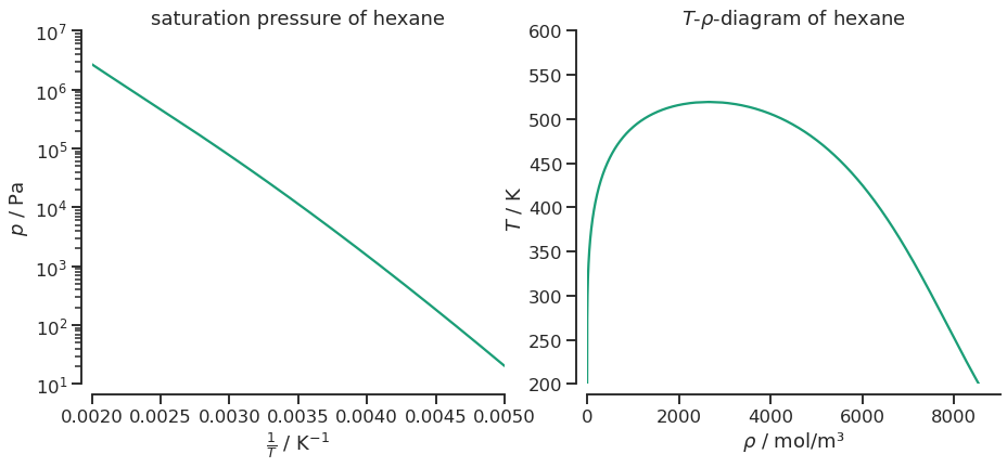
fig, ax = plt.subplots(1, 2, figsize=(15, 6))
ax[0].set_title(f"saturation pressure of {parameters.pure_records[0].identifier.name}")
sns.lineplot(y=df.pressure, x=1.0/df.temperature, ax=ax[0])

# axis and styling
ax[0].set_yscale('log')
ax[0].set_xlabel(r'$\frac{1}{T}$ / K$^{-1}$');
ax[0].set_ylabel(r'$p$ / Pa');
ax[0].set_xlim(0.002, 0.005)
ax[0].set_ylim(1e1, 1e7)

ax[1].set_title(r"$T$-$\rho$-diagram of {}".format(parameters.pure_records[0].identifier.name))
sns.lineplot(y=df.temperature, x=df['density vapor'], ax=ax[1], color=colors[0])
sns.lineplot(y=df.temperature, x=df['density liquid'], ax=ax[1], color=colors[0])

# axis and styling
ax[1].set_ylabel(r'$T$ / K');
ax[1].set_xlabel(r'$\rho$ / mol/m³');
ax[1].set_ylim(200, 600)
ax[1].set_xlim(0, 9000)

sns.despine(offset=10)

The PhaseEquilibrium object

A PhaseEquilibrium object contains two thermodynamic states (State objects) that are in thermal, mechanical and chemical equilibrium. The PhaseEquilibrium.pure constructor can be used to compute a phase equilibrium for a single substance. We have to provide the equation of state and either temperature or pressure. Optionally, we can also provide PhaseEquilibrium object which can be used as starting point for the calculation which possibly speeds up the computation.

vle = PhaseEquilibrium.pure(
    pcsaft,
    temperature_or_pressure=300.0*si.KELVIN
)
vle

	temperature	density
phase 1	300.00000 K	8.86860 mol/m³
phase 2	300.00000 K	7.51850 kmol/m³

The two equilibrium states can be extracted via the liquid and vapor getters, respectively. Returned are State objects, for which we can now compute any property that is available for the State object and the given equation of state.

liquid = vle.liquid
vapor = vle.vapor

assert(abs((liquid.pressure() - vapor.pressure()) / si.BAR) < 1e-10)
print(f'saturation pressure      p_sat(T = {liquid.temperature}) = {liquid.pressure() / si.BAR:6.2f} bar')
print(f'enthalpy of vaporization h_lv (T = {liquid.temperature}) = {(vapor.specific_enthalpy(Contributions.Residual) - liquid.specific_enthalpy(Contributions.Residual)) / (si.KILO*si.JOULE/si.KILOGRAM):6.2f} kJ/kg')

saturation pressure      p_sat(T = 300 K) =   0.22 bar
enthalpy of vaporization h_lv (T = 300 K) = 365.83 kJ/kg

If you want to compute a boiling temperature or saturation pressure without needing the PhaseEquilibrium object you can use the

• PhaseEquilibrium.boiling_temperature and

• PhaseEquilibrium.vapor_pressure

methods. Note that these methods return lists (even for pure substance systems) where each entry contains the pure substance property.

PhaseEquilibrium.boiling_temperature(pcsaft, liquid.pressure())[0]

$300\,\mathrm{K}$

The states method returns all PhaseEquilibrium objects from PhaseDiagram

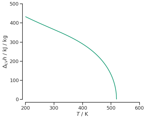
Once a PhaseDiagram object is created, we can access all underlying PhaseEquilibrium objects via the states field. In the following cell, we compute the enthalpy of vaporization by iterating through all states and calling the specific_enthalpy method on the vapor and liquid states of the PhaseEquilibrium object, respectively.

Note that this is merely an example to show how to compute any property of the states. The total value of enthalpy of vaporization may not be correct, depending on the ideal gas model used.

# Add enthalpy of vaporization to dataframe
df['hlv'] = [
    (vle.vapor.specific_enthalpy(Contributions.Residual) - vle.liquid.specific_enthalpy(Contributions.Residual))
    / (si.KILO * si.JOULE / si.KILOGRAM)
    for vle in phase_diagram.states
]

fig, ax = plt.subplots(figsize=(7, 6))
sns.lineplot(y=df.hlv, x=df.temperature, ax=ax)

# axis and styling
ax.set_xlabel(r'$T$ / K');
ax.set_ylabel(r'$\Delta_{LV} h$ / kJ / kg');
ax.set_xlim(200, 600)
ax.set_ylim(0, 500)

sns.despine(offset=10);